Differential expression is the question behind a huge fraction of RNA-seq experiments: which genes change between my conditions, and can I trust the change? The biology is usually clear in your head. The bottleneck is everything between a folder of count files and a figure you'd actually put in a paper.
This post walks through that journey the way it should feel — as a conversation about your experiment, not a fight with a programming environment.
What the analysis actually involves
Strip away the tooling and a standard bulk RNA-seq comparison is four steps:
- Quality control — confirm libraries are healthy and samples cluster the way you expect.
- Normalisation — make samples comparable so sequencing depth isn't mistaken for biology.
- Modelling — fit a statistical model (DESeq2, edgeR, limma-voom) that accounts for your design.
- Interpretation — rank genes by fold change and adjusted p-value, then visualise.
None of that is conceptually hard for a biologist. The friction is that each step traditionally means installing packages, matching versions, and writing code that breaks if a column name has a space in it.
Describe the comparison in plain English
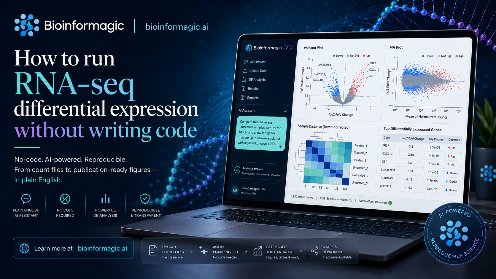
With Bioinformagic, you start where your thinking starts. Something like:
Compare treated versus untreated samples, control for batch, and show me the genes that go up or down with an adjusted p-value under 0.05.
From that sentence, the assistant assembles a real DESeq2 workflow: it reads your count matrix and sample sheet, sets the reference level, includes batch in the design formula, runs the model, and applies multiple-testing correction. You review each decision before anything runs — nothing is hidden.
You stay the scientist
The point isn't to remove you from the analysis. It's to remove the parts that were never really science — the dependency errors, the Stack Overflow detours, the half-remembered ggplot2 syntax. You still choose the contrast, the threshold, and the interpretation.
From model to figure
Once the model fits, you get the outputs you'd expect to hand a collaborator:
- A ranked results table with log2 fold changes and adjusted p-values.
- A volcano plot with significant genes highlighted.
- An MA plot and sample-distance heatmap for sanity checks.
- A short, readable summary of how many genes moved and in which direction.
Every figure is regenerated from the same pinned workflow, so the plot in your slide deck matches the numbers in your supplement.
Why "reproducible" matters here
Six months from now, a reviewer asks you to re-run the analysis with one sample removed. In the old world, that's a small panic: which package versions did you use, and does the script still run? Here, the workflow and its environment are captured together, so the re-run is one more sentence — "drop sample 7 and repeat" — not an archaeology project.
That's the whole idea: keep the rigour of a hand-written DESeq2 script, lose the part where reproducing it depends on remembering exactly what you did.
Try it on your own data
If you've been waiting on a bioinformatician to run a comparison you could describe in a sentence, this is built for you. Join the early-access list and bring a dataset you already understand — it's the fastest way to see whether the results match your intuition.